Ranking the Perceived Safety of Streets
Using crowd-sourced comparisons of street view images, I explored how people perceive safety in urban environments. By combining a large dataset with modern computer vision techniques, I trained a model that can rank streets based on how safe they appear.
I’ve always been curious about how we visually perceive streetscapes. In an earlier project, I built a deep learning model to segment features like roads, sidewalks, and sky, and used this information to estimate the overall “quality” of a street. This idea isn’t new. For example, Naik et al. (2014) at MIT Media Lab developed a StreetScore algorithm that used regression models and generic image features to predict perceived street safety. Later, Ma et al. (2020) applied semantic segmentation to classify elements such as trees, buildings, and pavement, creating indexes based on the proportion of pixels each feature occupied in an image. Related measures like the “green view” and “sky view” indexes were also used in the Global Streetscapes project by Hou et al. (2024).
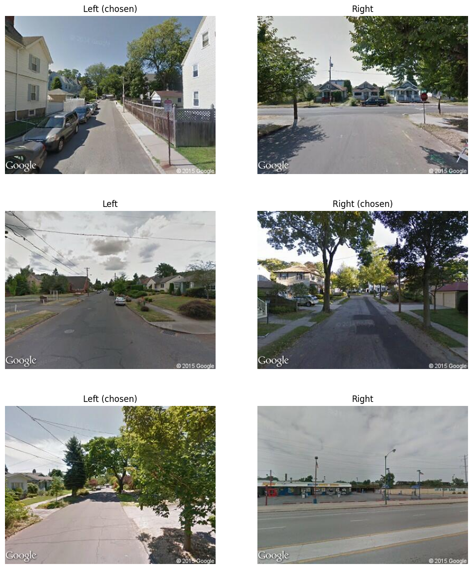 Sample of pairwise comparisons in Place Pulse 2.0 dataset
I wanted to build on this line of work using the Place Pulse 2.0 dataset, introduced by Dubey et al. (2016), to train a model that ranks street view images across six attributes: safe, lively, boring, wealthy, depressing, and beautiful. Place Pulse 2.0 is a large dataset, with 1,170,000 pairwise comparisons between 110,988 Google Street View images collected from 56 cities over 33 months. Participants were asked to compare two images at a time on one of the six attributes. One limitation however is that the paper doesn’t clearly define what “safety” means. Whether it refers to personal safety or safety related to walking, biking, or other modes of travel. Still, the authors note strong correlations between safety and beauty, as well as safety and liveliness, supporting ideas in urban design that link safer streets with more vibrant environments.
Using the pairwise comparisons they used the TrueSkill ranking algorithm to generate scores for each of the images between 0 and 10. However the main challenge with that method is that any given image needs roughly 24-36 comparisons to achieve stable rankings. This would require 1.2 to 1.9 million comparisons per attribute!
Ranking vs Scoring
Dubey did find a unique way to get around the limited pair wise comparisons. They trained a binary classifier (using both a ranking algorithm and classification siamese network) to predict the preferred image for any given attribute and generated synthetic data. The additional data could the be used to determine TrueSkill values for each image which could then be fed into a regression model. This brings up an interesting discussion on the bias introduced by regression vs. a simple ranking model as suggested by Porzi (2015). Choosing to fit a regression model to an arbitrary scoring function like TrueSkill doesn’t reflect the true user judgement of images. Ranking may be more appropriate because it’s using the original pairwise judgement reducing the bias introduced by a scoring function.
How can we rank (and score) streetscapes?
There are inherent qualities that we perceive from a street that help us judge how we feel about it. Do we feel safe, scared, inspired, at ease or welcomed? Ewing and Handy (2009) had described five perceptual qualities that describe walkable streets: imageability, enclosure, human scale, transparency and complexity. Imageability refers to the ability of a street to create a strong mental image and sense of place, with distinct features that stand out and are easy to recognize. Enclosure describes how blocked sight lines can make outdoor spaces feel like safe, room-like environments that people remember positively. Human scale ensures that buildings and structures are kept within proportions that feel approachable and comfortable for people. Transparency captures both the physical openness of spaces, such as light passing through windows or visible entryways, and the social signal of human activity on the street. Finally, complexity reflects the variety of visual and sensory details like architecture, signage, people, textures, and light that make a streetscape engaging and lively.
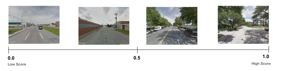 Scoring streetview images can help us rank them according to perceived safety
The task of ranking inputs falls under Learning to Rank (LTR), a machine learning approach for training models to assign scores that minimize a defined loss function. LTR has been widely applied in search engines and recommender systems. Training methods generally use pointwise, pairwise, or listwise loss functions. The LTR objective is to produce an ordinal ranking and therefore scoring of the perceived safety of streetview images in the Place Pulse 2.0 dataset.
For our Place Pulse 2.0 dataset, we require a pairwise method that predicts relative preference. Given two images, the goal is to determine which one ranks higher. Dubey applied RankSVM, which relies on a squared hinge loss. However, a more common approach is RankNet, which uses binary cross-entropy loss. RankNet provides smoother gradients, better generalization, and greater noise tolerance than RankSVM.
Extensions such as LambdaRank and LambdaMART further improve upon RankNet, but given the simplicity of implementation, we will adopt RankNet as our loss function moving forward.
In RankNet, The model estimates the probability that the left image, \(i\) should be ranked above the right \(j\). We’re basically passing the difference between the left image score and right image score \(s_i-s_j\) into a sigmoid function:
\[ P_{ij} = \frac{1}{1 + e^{-(s_i - s_j)}} \]
We then use the probability with binary cross entropy loss:
\[ L_{ij} = - \Big( y_{ij} \, \log P_{ij} + (1 - y_{ij}) \, \log (1 - P_{ij}) \Big) \]
Where the the ground truth labels are 1 if left image, \(i\) should be ranked above the right \(j\) and 0 otherwise.
Model Architecture
To train our model, we first require input features that can be optimized under the RankNet loss function. For this purpose, we use Meta’s DINOv3 Vision Transformer, an evolution of DINOv2, which produces robust, high-quality representations suitable for downstream tasks with little or no fine-tuning.
Specifically, we leverage the [CLS] embedding, a global feature vector that captures high-level semantic information about an image. In the context of street-view imagery, this embedding can be thought of as encoding the overall “vibe” of a street.
Using this embedding as input to a simple linear probe (a linear layer), we predict a scalar score for each image. These scores are then compared pairwise using the RankNet loss to train the ranking model.
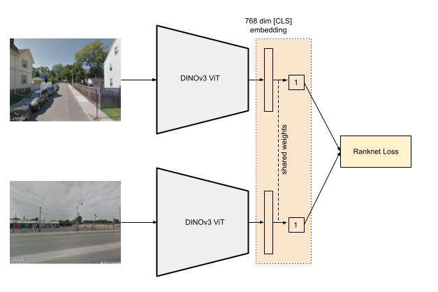
Architecture using DINOv3 embeddings, linear probe and RankNet loss function
Dataset Cleaning
Pairwise ranking of this sort of data can include a lot of noise so to maintain a clean set of data we need to filter down the original 1.1 million pairwise comparisons. Since we’re only using a linear classifier for training with only 768 parameters we won’t need much data so we can be selective in what we use. The safety attribute had the highest number of pairwise comparisons so we only include those rows. The original dataset included street view images from 56 cities. Let’s just include the North American cities: Toronto, San Francisco, Portland, Philadelphia, Montreal, Minneapolis, Los Angeles, Houston, Atlanta, New York, Denver, Chicago and Boston. That filters data down to 39,920 comparisons. We can reduce further by filtering out images that are really similar to each other and would create additional noise in the dataset. To do this we can use the same DINOv3 embeddings for each set of pairs and determine the cosine distance and filter any pairs less than a threshold.
| left                         | right                        | cosine_distance |
|------------------------------|------------------------------|-----------------|
| 513d9c83fdc9f03587007d7a     | 5185d46bfdc9f03fd50013d5     | 0.216851        |
| 51413ae5fdc9f04926005812     | 5185d46bfdc9f03fd50013d5     | 0.219624        |
| 513d7eecfdc9f035870074e6     | 5185d46bfdc9f03fd50013d5     | 0.155212        |
| 513cc9f6fdc9f03587001ca0     | 513cbed8fdc9f035870011fe     | 0.130798        |
| 50f607e0beb2fed6f800037d     | 50f6086ebeb2fed6f800048d     | 0.228235        |
Filtering out rows with cosine distance less than 0.20, we’re finally left with 18,961 high quality pairwise comparisons.
Using HuggingFace to Train
The Hugging Face transformers library offers a simple way to access pre-trained models and image processing. By extending the PreTrainedModel class we can free the ViT parameters, add the linear classifier and forward pass the CLS embedding.
class DinoV3Ranker(PreTrainedModel):
  config_class = DINOv3ViTConfig()
  base_model_prefix = "backbone"
  def __init__(self, config):
    super().__init__(config)

    self.backbone = DINOv3ViTModel(config)
    for param in self.backbone.parameters():
      param.requires_grad = False

    hidden_size = self.backbone.config.hidden_size
    self.classifier = nn.Linear(hidden_size, 1) #Linear probe

  def forward(self, pixel_values):
      outputs = self.backbone(pixel_values=pixel_values, return_dict=True)
      cls = outputs.last_hidden_state[:, 0, :]  # cls embedding
      score = self.classifier(cls).squeeze(1) # cls embeddings
      return score
Then instatiating the model is simple:
config = AutoConfig.from_pretrained("facebook/dinov3-vitb16-pretrain-lvd1689m")
model = DinoV3Ranker(config).from_pretrained("facebook/dinov3-vitb16-pretrain-lvd1689m")
The custom RankNet loss function can be added in compute_loss:
def compute_loss(self, model, inputs, return_outputs=False, num_items_in_batch=None):
    left_pixel_values = inputs["left_pixel_values"]
    right_pixel_values = inputs["right_pixel_values"]
    labels = inputs["labels"].float()

    r_i = model(left_pixel_values)
    r_j = model(right_pixel_values)

    # RankNet probability that r_i > r_j
    p_ij = torch.sigmoid(r_i - r_j)

    # Binary cross-entropy loss
    loss = F.binary_cross_entropy(p_ij, labels)

    outputs = torch.stack([r_i, r_j], dim=1)  # for metrics
    return (loss, outputs) if return_outputs else loss
Training for around 5 epochs, we get an acceptable (but not state of art) AUC measure of 0.76. Enough to see if the model is learning anything useful.
You can find the entire training script and Jupyter notebook here.
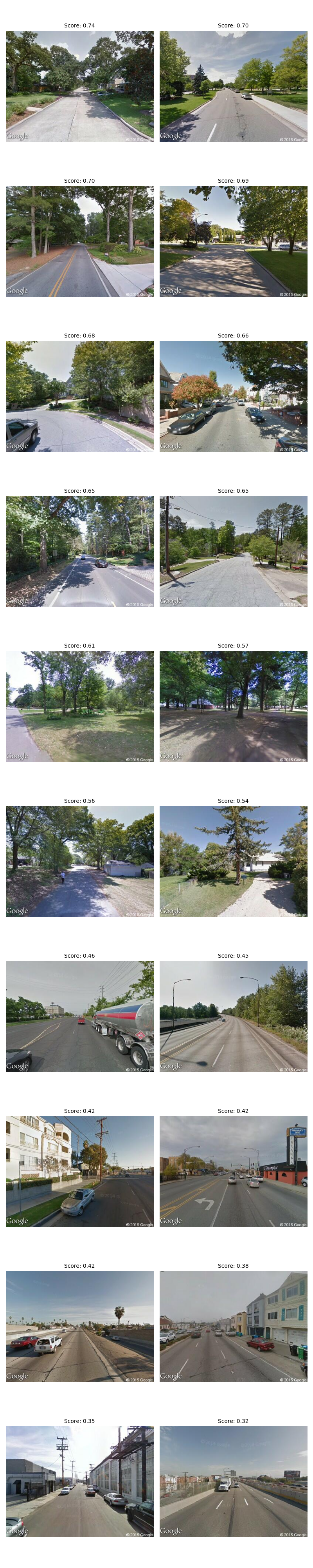
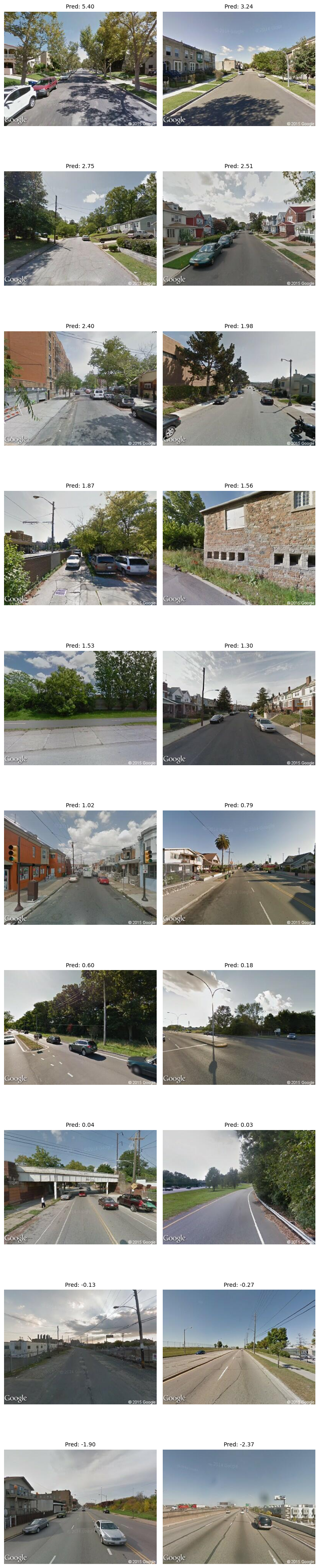
Inference Results
Running inference on the test set, we can get scores for individual street view images and then order them. Higher score values correspond with high perceptions of safety and walkability.
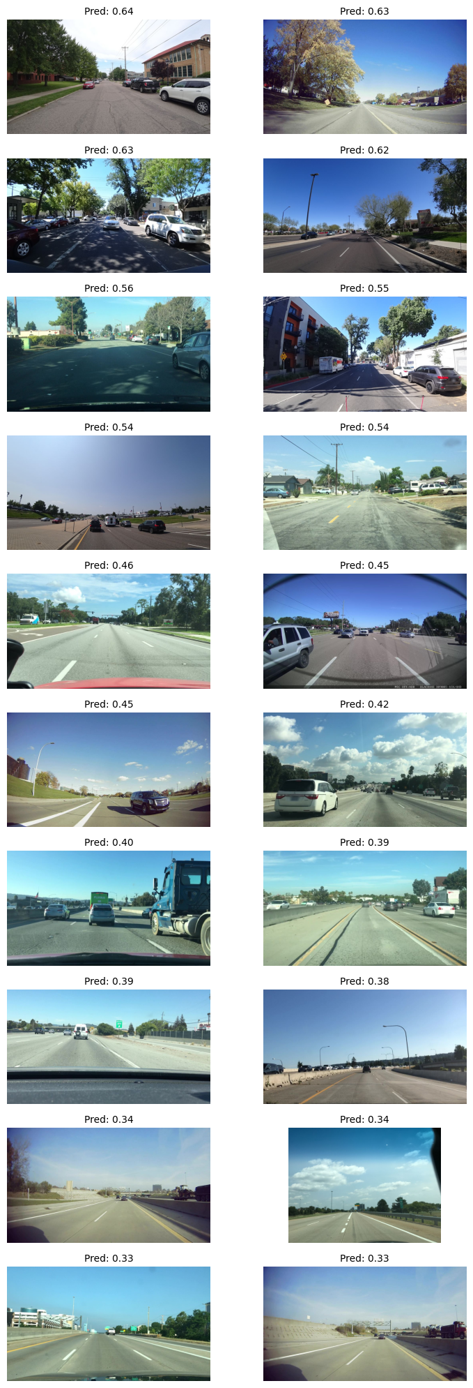
Inference on Mapillary Images
Running the model on Mapillary street view images would obviously produce sub par results since the the input images are not from the same distribution (or the same quality) as Google Street View. But it’s still interesting to see what the model will output. We can see right away that although the ordering somewhat makes sense and maintain a logical ordering but the scoring values distribution differs from the Google Street View images.
I ran this set of inference on the Global Streetscapes benchmark dataset where we’re able to filter the imagery according to a set of quality criteria (i.e. front facing, daylight, etc.)
Ranking using Steering Vector
I found an interesting paper from some authors out of Tübingen AI Center titled “On the rankability of visual embeddings” by Sonthalia (2025). Instead of training a ranking model, the authors demonstrate that using a small number (or often two extreme) examples can be enough to determine a rank axis for an embedding. They describe one method as “Few-shot learning with extreme pairs”.
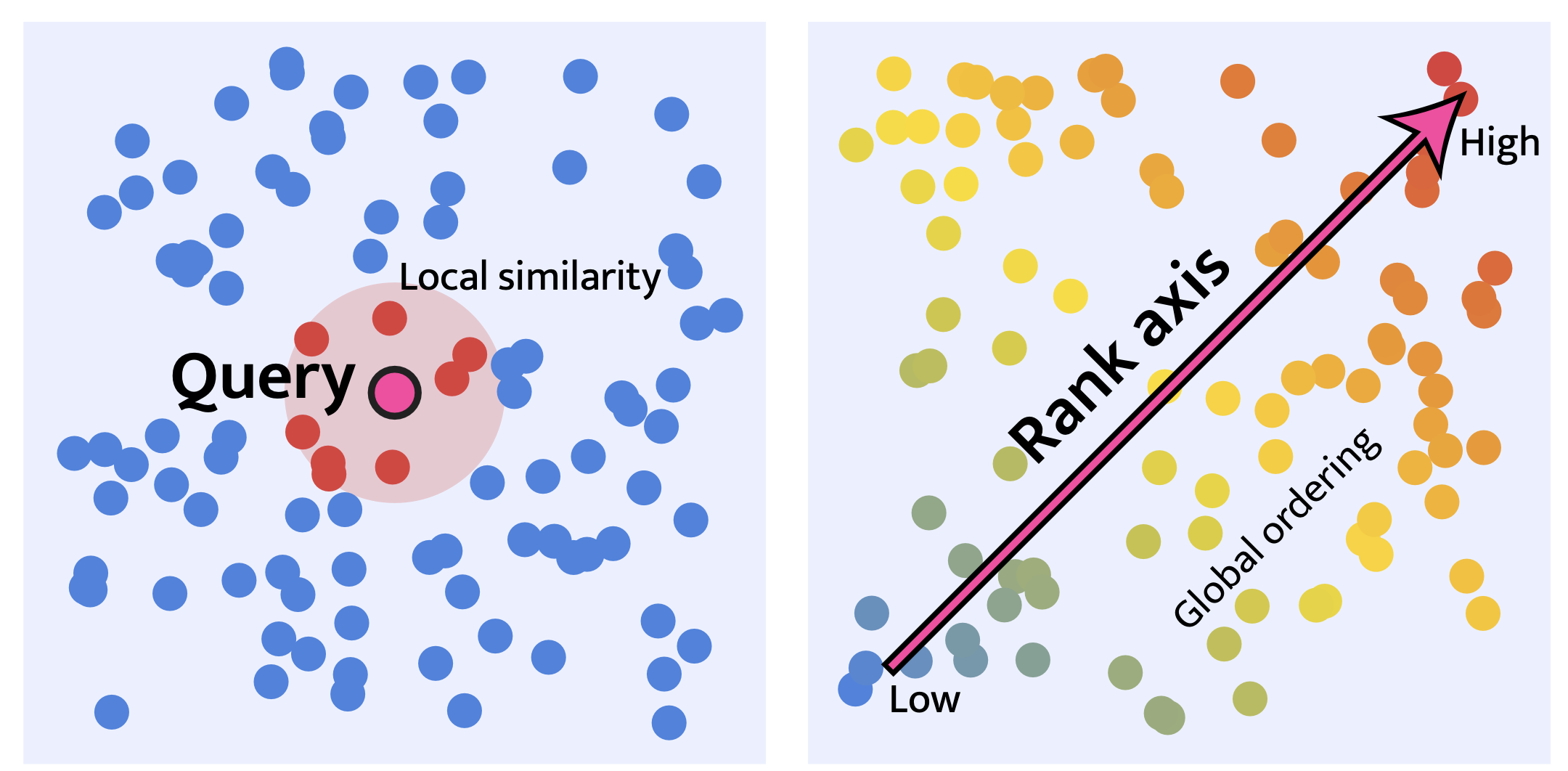 Retrieval (left) vs. Ranking (right) taken from Sonthalia (2025)
In the case of our street view images, we could find a sample low safety, \(x_l\) and high safety image, \(x_u\) and use them to determine a steering vector. The steering vector is calculated by subtracting the lower bound embedding from upper bound embedding and divide by the norm of the two embeddings:
\[ v_A = \frac{x_u - x_l}{\lVert x_u - x_l \rVert} \]
![]() Hand picked extremes used to calculate the steering vector
Hand picked extremes used to calculate the steering vector
Results
Now if we multiply the steering vector by an image embedding we can get a ranking score \(r = v_A^{\top} x\). The results are surprisingly good and align with the RankNet model however the scalar values are arbitrary where RankNet is constrained by the sigmoid function to between 0 and 1. Using hand picked extreme values does introduce bias in the ranking method however it does allow us to fine tune the rank axis according to a specific application for example, walkability or bikeability,
References
Ewing, R., & Handy, S. (2009). Measuring the Unmeasurable: Urban Design Qualities Related to Walkability. Journal of Urban Design, 14(1), 65–84. https://doi.org/10.1080/13574800802451155
Dubey, A., Naik, N., Parikh, D., Raskar, R., & Hidalgo, C. A. (2016, September). Deep learning the city: Quantifying urban perception at a global scale. In European conference on computer vision (pp. 196-212). Cham: Springer International Publishing.
Hou Y, Quintana M, Khomiakov M, Yap W, Ouyang J, Ito K, Wang Z, Zhao T, Biljecki F (2024): Global Streetscapes – A comprehensive dataset of 10 million street-level images across 688 cities for urban science and analytics. ISPRS Journal of Photogrammetry and Remote Sensing, 215: 216-238. https://doi.org/10.1016/j.isprsjprs.2024.06.023
Ma, X., Ma, C., Wu, C., Xi, Y., Yang, R., Peng, N., Zhang, C., Ren, F. (2021). Measuring human perceptions of streetscapes to better inform urban renewal: A perspective of scene semantic parsing. Cities, 110, 103086.
Naik, N., Philipoom, J., Raskar, R., Hidalgo, C. (2014). Streetscore – Predicting the Perceived Safety of One Million Streetscapes. 2014 IEEE Conference on Computer Vision and Pattern Recognition Workshops, Columbus, OH, USA, 2014, pp. 793-799, doi: 10.1109/CVPRW.2014.121.
Porzi, L., & Lepri, B. (2015). Predicting and Understanding Urban Perception with Convolutional Neural Networks. Proceedings of the 23rd Annual ACM Conference on Multimedia. https://doi.org/10.1145/2733373.2806273
Sonthalia, A., Uselis, A., Joon Oh, S. (2025). On the rankability of visual embeddings. arXiv preprint arXiv:2507.03683. https://doi.org/10.48550/arXiv.2507.03683