Measuring Transit Reliability with Open Data: A Cloud-Based Approach to On-Time Performance
Transit riders judge reliability not just by frequency, but by whether buses actually arrive when the schedule says they will. Using open GTFS and GTFS-Realtime data, I set out to measure on-time performance (OTP) using data collected with a cloud-based ETL pipeline. This approach makes transit reliability analysis transparent, scalable, and reproducible.
Transit agencies around the world rely on different measures to evaluate how reliable their service is. In North America, the most widely used metric is on-time performance (OTP). This measure captures how well a bus service adheres to its published schedule. Although it may differ agency to agency , a bus is typically considered on time if it arrives at a stop between 1 minute early and 5 minutes late of the scheduled time. OTP remains popular because it is straightforward to calculate and can be aggregated across an entire system.
Most transit agencies today have Computer-Aided Dispatch and Automatic Vehicle Location (CAD-AVL) system that collect high resolution telemetry and vehicle data. Historical CAD-AVL records are not often published to open data websites so it’s difficult calculate OTP independently. I wanted to see how I could build a ETL (extract, transform and load) pipeline using cloud services and publicly available GTFS and GTFS-Realtime datasets to determine stop level OTP.
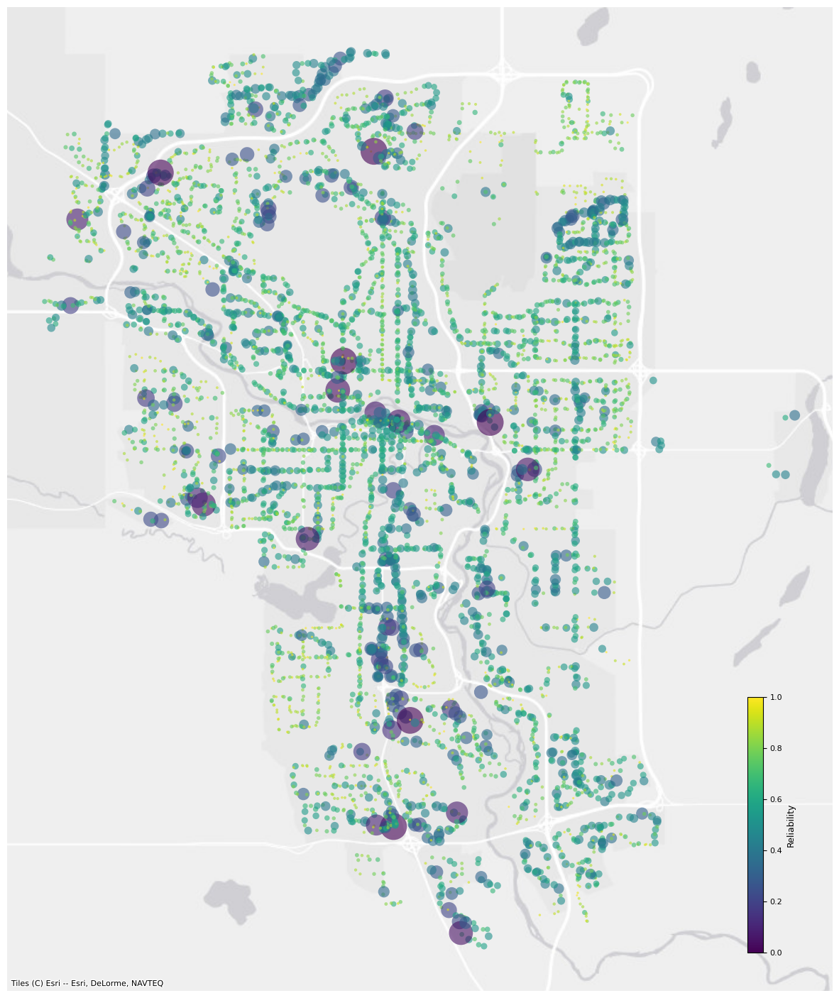 Stop level reliability for Calgary Transit using data collected between November 1 and November 9, 2024. This is the probability that a bus will arrive between one minute early and five mins late from the stop time. Larger circles mean lower reliability.
Building a Data Collection Pipeline
To calculate OTP in Calgary, both GTFS Static data (published schedules) and GTFS Realtime data (actual bus positions) were needed. Because historical CAD-AVL data isn’t available, I created a custom extract, transform, load (ETL) pipeline using Amazon Web Services (AWS). You can find the code for the ETL pipeline here.
The architecture, shown below, continuously gathered bus positions for the entire system every 60 seconds and stored them in a database:

AWS ETL Architecture diagram
Here’s how it worked step by step:
- EventBridge Scheduler – Triggers the process every minute to fetch new GTFS Realtime vehicle position data.
- Lambda Function – A serverless compute resource that requests the GTFS-RT feed, parses the raw data, and formats it for storage.
- Internet & NAT Gateway – Provide secure connectivity for the Lambda function to access the GTFS feed while remaining inside a VPC (Virtual Private Cloud).
- Amazon RDS (PostgreSQL) – Stores parsed records including:
- Timestamp (datetime)
- Trip ID
- GPS latitude and longitude
One limitation of using AWS EventBridge is that it doesn’t provide second level precision for the scheduler; the minimum resolution is one minute. Some transit agencies, including Calgary Transit have 15 second resolution for their vehicle positions meaning we are missing some of the data in our ETL pipeline. To achieve sub minute schedules, other services would be needed such as Step Functions or an EC2 Instance.
This design was both scalable and automated, capable of handling millions of records without dedicated servers. Between November 1 and November 9, 2024, the pipeline collected over 2 million records. It cost approximately $10 USD to operate the AWS services listed above during that period.
From Raw Data to Schedule Deviations
Once the data was collected, the next step was to measure how actual arrivals compared to scheduled ones. Using the GTFS Static schedule, a query was run to find all vehicle location points within a 15m buffer of a stop location for a given trip.
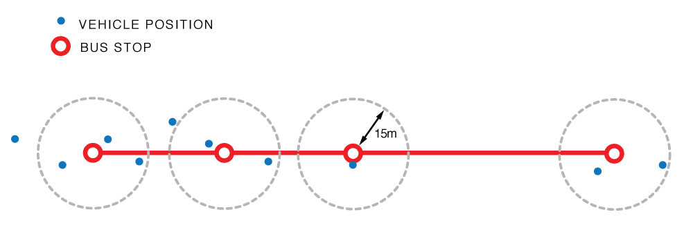
Vehicle positions within a 15m radius of the bus stop
For each stop and trip:
- The first matching vehicle position was selected.
- A schedule deviation was calculated: observed datetime minus scheduled stop_time.
- Outliers beyond ±15 minutes were filtered out.
- Deviations were averaged across stops to obtain both the mean and standard deviation for each stop.
This process provided a stop-level dataset of schedule deviations across the entire system.
| stop_id | count |    avg    |   stddev   |     long     |     lat     |  z_min   |  z_max   | reliability |
|---------|-------|-----------|------------|--------------|-------------|----------|----------|-------------|
| 1900    | 43    | 182.418605| 95.849891  | -113.949496  | 51.132644   | -1.903170| 1.226724 | 0.861528    |
| 1901    | 4     | 86.750000 | 92.272694  | -113.980664  | 51.131861   | -0.940148| 2.311085 | 0.816015    |
| 1903    | 29    | 79.344828 | 81.893343  | -113.959360  | 51.158135   | -0.968880| 2.694421 | 0.830172    |
| 1904    | 47    | 79.085106 | 74.195637  | -113.961301  | 51.158173   | -1.065900| 2.977465 | 0.855312    |
| 1905    | 30    | 85.833333 | 72.416460  | -113.962564  | 51.156819   | -1.185274| 2.957431 | 0.880494    |
Computing On-Time Performance
With average schedule deviation and standard deviation, OTP was computed using a cumulative density function (CDF). For each stop the probability that a bus arrived between -1 minute (−60 seconds) and +5 minutes (300 seconds) of the scheduled time was calculated:
\[ OTP_{\text{stop}} = P(S_{-1} \leq T \leq S_{5}) = F(300) - F(-60) \]
We can do this by calculating the min and max z-scores and then subtract them:
\[ z = \frac{x - \text{avg}}{\text{std}} \]
Calculating the z-score for the minimum (-60 seconds arrival) would be:
\[ z_{min} = \frac{-60 - \text{avg}_{\text{stop_id}}}{\text{std}} \]
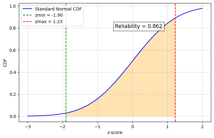
Sample reliability for a given stop. Subtracting the z-scores give us the probability that a bus will arrive between -1 minute (−60 seconds) and +5 minutes (300 seconds) of the scheduled time
Reliable transit service is not just about how often buses run it’s about whether riders can trust the schedule. By using open GTFS data and cloud infrastructure, I wanted to demonstrate how to measure OTP in a transparent, scalable way that can be replicated for any transit agency.