Pedestrian Collision Hot Spot Detection Using Machine Learning and Embeddings
Cities in North America have adopted vision zero policies with the goal of eliminating all traffic fatalities and injuries. There’s no doubt that the design of transportation infrastructure plays a major factor in collision occurrence. How can machine learning and geospatial embeddings play a role in predicting hot spots based on infrastructure design and other geographic features?
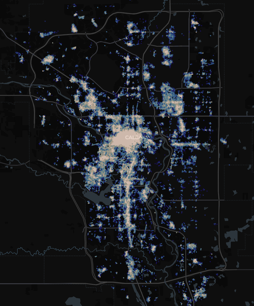 Prediction of pedestrian collision hot spots in Calgary. You can find jupyter notebooks of this work on github
Despite efforts to reduce pedestrian collision fatalities and injuries through policy or safety regulations, the disappointing fact is that they have gradually increased over the past 40 years. Increasingly large SUVs and trucks as well as distracted driving are some suspected factors contributing to this. Vision Zero is a movement started in the late 90s with the aim of eliminating all traffic related injuries and fatalities. Its popularity in recent years has resulted in mainstream adoption in most major cities in North America. This map shows all the cities in Canada that have adopted Vision Zero policies. But, despite best efforts, collision fatalities and injuries have proven a stubborn trend to control.
Contents
- Machine Learning & Collision Prediction
- Prediction Results
- Feature Engineering
- Using Embeddings
- Training Results
Machine Learning and Collision Prediction
Road design undoubtedly plays one of the biggest roles. Slip lanes, wide and numerous crossing lanes, high speed limits, lack of cross walks, poor visibility, narrow sidewalks, no sidewalks, the list goes on. Arterial roadways that traverse high density nodes or corridors also increase the chance pedestrian contact with vehicles.
What role can geospatial data science play in understanding how these road designs and other urban features affect the probability of collisions?
I explored this relationship using the traffic “incident” dataset in Calgary. The dataset covers all road incidents including stalled vehicles, vehicle collisions as well as pedestrian collisions. My goal was to develop a toy binary classification machine learning model that predicts the probability of a pedestrian collision occurrence across Calgary given some input temporal (month, hour of day and day of week) and geographic features (OSM tags). The output is a map that shows hot spot pedestrian collision locations across the city at various times. In this post I explore my methodology and the key idea of using embeddings (thanks to the recently released srai python package) to help train machine learning models for geospatial tasks.
You can find the jupyter notebooks of this work on github.
Prediction Results
Predictions across a temporal ranges sometimes do not show much variability. As expected the regions that show the most intensity of collisions are in highly dense areas like downtown Calgary, and activity nodes like the educational institutions (schools, colleges, universities) and shopping centres (Sunridge, Marlborough, Chinook)
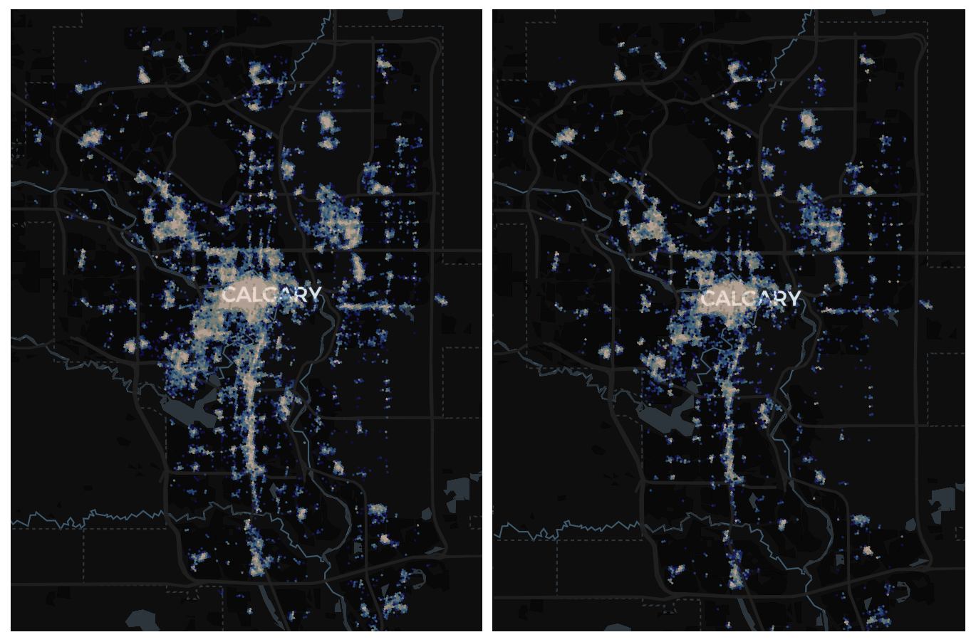 Above: Prediction for September 9am (left) and 5pm (right). There is not much change in intensity between morning and evening rush hour with a very minor decrease shown in the 5pm prediction.
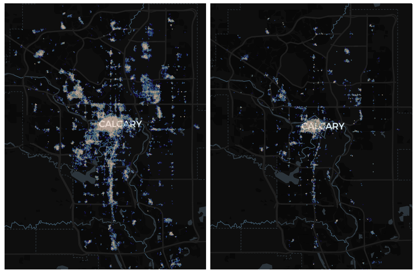 Above: Prediction for February 9am (left) and 5pm (right)
Road features that we expect to be the highest risk were picked up by the model, often highlighting intersections that had slip lanes and that were also close to dense pedestrian activities such as shopping centres or schools.
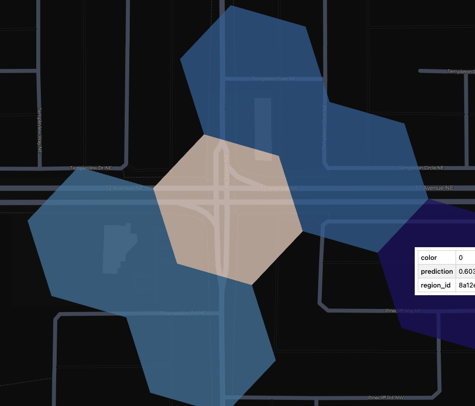 The model highlights slips lanes (highlighted in white hexagon) near high density areas (schools, shopping centres, etc.) consistently as areas of high pedestrian collision probability.
Feature Engineering
Feature engineering latitude and longitude coordinates for machine learning tasks can be challenging. Latitude and longitude represent a location on a sphere so they cannot simply be used as is since the proximity of points are not represented in the data (i.e. 0 and 180 degrees longitude are adjacent). Even if the coordinates were transformed into something feasible that represented a spherical pattern (this is often a useful trick), it would be difficult to train a linear model given the precision and variance of the coordinates.
Above: A one hot encoded geospatial feature will result in a far too many dimension resulting in the “curse of dimensionality”. We typical won’t have enough data to train with that many features.
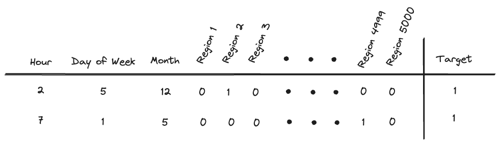
Clustering or binning is often a solution to this. Clustering methods can be used to group collections of coordinates. Depending on the number of clusters and the task at hand this may not be a suitable solution since predictions may be for very coarse resolutions (large geographic areas) and not useful for practical applications. S2, Geohash or H3 are grid systems that can be used for binning geospatial coordinates. The region indices can then be used as categorical features in a model. Depending on the resolution of the grid system, the number of unique categories may become unmanageable. The number of regions covering a city for example could number in the hundreds or thousands. One-hot encoding such a large number of features makes machine learning tasks difficult because it introduces the curse of dimensionality. It’s often difficult to find enough data to cover so many features and train accurately.
Coordinates can be grouped by H3 regions. Each region can be used as a feature in a machine learning model however one-hot encoding a very large number of regions becomes problematic.
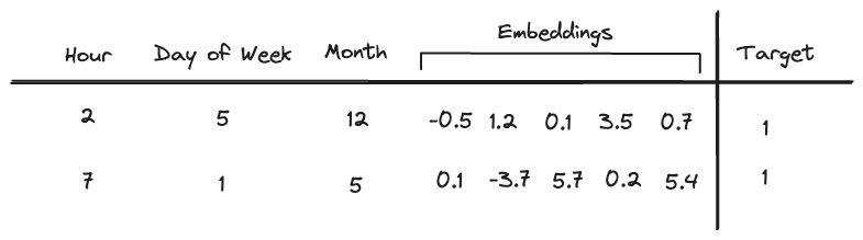
Above: Embeddings are a more expressive way to represent geographic data, for example through OSM tags.
Using Embeddings
Embedding help address many of the problems mentioned above by using a compact vector representation of spatial features that can then be fed into machine learning tasks. Embeddings have become popular in recent years in the field of Natural Language Processing (NLP) and form a crucial step in any NLP task.
For geospatial or location data, embeddings are an emerging area of research that show improvements in geospatial ML tasks. Loc2Vec, Hex2Vec, Space2Vec, Urban2Vec and GeoVeX are some models that have emerged in literature recently with a few implemented in the recently released Spatial Representations for Artificial Intelligence (SRAI) python library.
Loc2Vec
First proposed by location insights company Sentinence, Loc2Vec uses rasterized OSM map data to create a 12 channel (each channel extracts certain geographic features such as roads, building, etc.) tensor that is input into a convolutional encoder network. The model uses concepts from computer vision and is trained in a self supervised manner using a triplet loss function.
 Source: https://sentiance.com/loc2vec-learning-location-embeddings-w-triplet-loss-networks
Hex2Vec
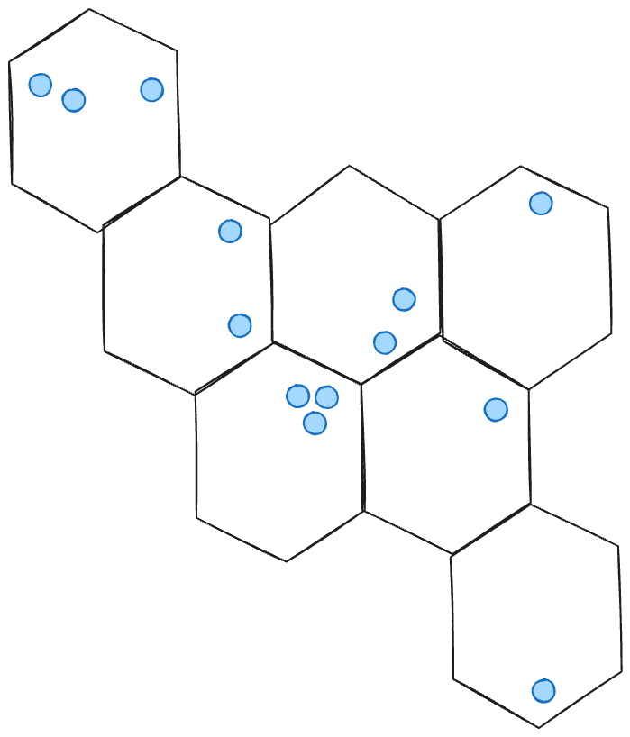
Developed by Wrocław University of Science and Technology researchers Wozniak & Szymanski, Hex2Vec uses H3 spatial indexes to count OSM tags for a given region and then uses a skip gram model with negative sampling to train embeddings. The context regions were chosen immediately adjacent to a target region, while negative regions sample are chosen from any area not including the target or context.
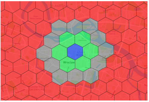
Above: Target (blue), context (green) and negative (red) sampling regions for Hex2Vec in Wozniak & Szymanski (2021).
GeoVex
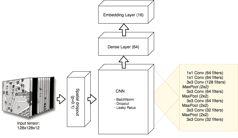
The GeoVex model, developed by data scientists at Expedia Group, uses H3 spatial indexes and OSM tags to describe a k-dimensional histogram with the frequency that a tag occurs in a given index. A novel Hexagonal Convolutional Autoencoder combined with a Zero-Inflated Poisson (ZIP) reconstruction layer is used to generate embeddings. GeoVeX is unique because it uses a convolutional approach to take into account context from neighbouring H3 regions.
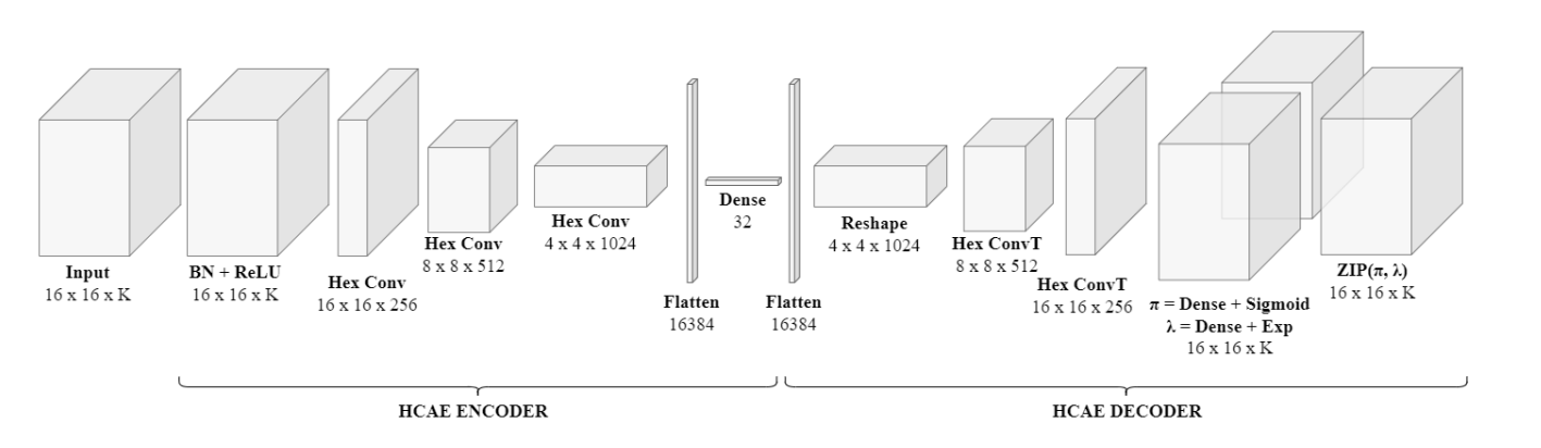
Above: Model architecture used for GeoVex.
Training Results
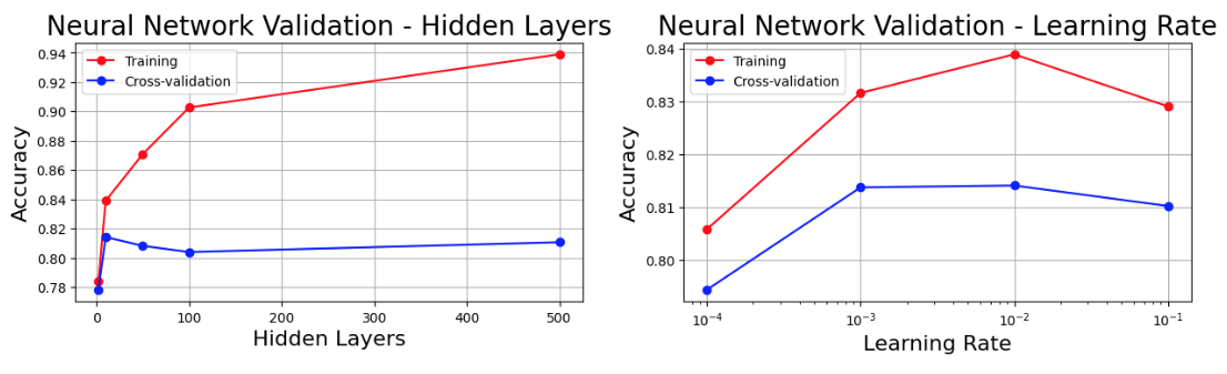
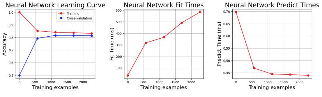
The pedestrian collision hot spot detection task above used GeoVex embedding at a 10-depth H3 resolution. Using a 5 dimension embedding, we can simply use a linear classifier to train our model. Using sklearn MLPClassifier with a single layer, preserving the probability outputs and predicting over all regions of the city, the result is a probability map that shows the highest probability pedestrian collision locations given some input features - hour of day, day of week and month. The original dataset contained around 1510 instances of pedestrian collisions, however this was expanded to 3020 to also include negative targets (locations where there was no collision). Accuracy on the test data is around 85%. The validation and learning curves are shown below using 5 fold cross validation on the test set.
You can find jupyter notebooks on github to reproduce the results.
Discussion
-
The negative sampling approach involved randomly selecting road locations along the OSM network and then using a perfectly balanced split between positive (collision locations) and negative (no collision locations) targets. This was used to simplify the experiment and help in validation. Considering that collisions in general are relatively low probability events, the balanced strategy does not reflect the actual distribution of collisions occurring. A more appropriate strategy may be to over sample the negative targets and use sample weights for training.
-
The OSM tags used in the GEOFABRIK layer are exhaustive. The selected tags will impact the model results. I didn’t fine tune the selected tags and this may require some experimentation to see how it impacts the model.