Segmenting Street-Level Images with Computer Vision using Tensorflow
In this post I outline my workflow in training a toy convolutional neural network (CNN) model from start to finish including creating my own ground truth images. The model is then used to predict semantic segmentation masks of street-level images, a tool popular in autonomous vehicle driving applications.
For this exercise, I’m working with 100 Google Street View images divided into 80 images for training and 20 images for test. Using so few images will not produce a performant model, but this exercise was mainly to familiarize myself with the general CNN training workflow as well as Tensorflow’s data pipeline.
This post is divided into the following sections:
- Image Labelling (Ground Truth)
- Creating Image Label Masks
- Input data/image pipeline & creating TFRecords
- Building the Model
- Training the Model
- Prediction
Semantic segmentation, in a machine learning context, involves predicting and classifying each pixel in an image according to a set of labels. Before the popularity of deep learning, there weren’t many tools (at least available to your average computer vision enthusiast) that could help us successfully segment parts of an image. The OpenCV library was once popular and used methods such as thresholding, achieving variable results. Other traditional ML algorithms were too slow for any meaningful applications. Computer vision, with the help of Deep Learning, has made tremendous progress in segmentation tasks. Not only can we now segment complex images, but the prediction is near real time and highly accurate.
1. Image Labelling (Ground Truth)
Before beginning to train your model you need a dataset of images and corresponding ground truth labels. Image labelling can be one of the biggest roadblocks to getting started training your own computer vision or segmentation model. It involves outlining individual objects in an image by drawing polygons - a time consuming and tedious process. Finding an application or platform to label your images is another hurdle and can be quite confusing. There are a handful of applications, both fee based and open sourced, that do an adequate job of the task:
Each application has varying qualities of UI and usability and it’s best to find one that suits your labelling needs and workflow. You must also be familiar with some of the image annotation formats such as PASCAL VOC, COCO, etc used by popular image datasets. PASCAL VOC uses XML while COCO uses JSON for example. It ultimately doesn’t matter which you use as long as you can convert the polygon points into a mask image.
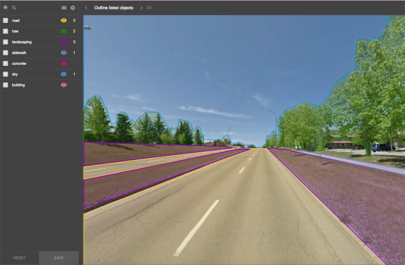 Labelbox interface
I used Labelbox to label 100 street images which took about 3 weeks of casual labelling in my free time. I used the following labels:
- Road
- Sidewalk
- Landscaping
- Tree
- Sky
- Concrete (bridge, barrier, median)
- Building
- Background
2. Create Image Masks
The next step involves creating label mask image files. In the label mask, each pixel corresponds to a label as outlined above. For example a sidewalk pixel would be labeled as a 2 and road pixel would be 1 and so on. The resulting mask would have each pixel in the image labelled. If you opened the file in photoshop you would see a black/grey image but if you inspected a particular pixel you could see the corresponding label as a RGB value (I.e. (1,1,1)). I used Labelbox and the PASCAL VOC specification and python PIL package to create the masks. Here is my simple script to save the masks as png files.
classes = {
  "tree":(1,1,1),
  "landscaping":(2,2,2),
  "road":(3,3,3),
  "sidewalk":(4,4,4),
  "building":(5,5,5),
  "sky":(6,6,6),
  "concrete":(7,7,7)
}

for mask in xml_mask:

  root = ET.parse(mask).getroot()

  width = int(root.find("size").find("width").text)
  height = int(root.find("size").find("height").text)

  img = Image.new("RGB", (width*2, height*2), 0) #scaling by 2 so
  #we can increase resolution and use anti-aliasing

  for objects in root.findall("object"):

    object_class = classes[objects.find("name").text]

    for object in objects.findall('polygon'):
      points=[]
      for element in object.findall('*'):
          points.append(element.tag)

      polygon = []
      for point in range(0, len(points) - 1, 2):
          x = int(object.find(points[point]).text)*2
          y = int(object.find(points[point + 1]).text)*2
          point = (x,y)
          polygon.append(point)
      ImageDraw.Draw(img).polygon(polygon, \
      fill=object_class,outline=object_class)
3. Building the Model
The next step involves choosing a CNN architecture appropriate for semantic segmentation. Typical networks that include convolution layers followed by fully connected layers, popular for image classification tasks, don’t work well with semantic segmentation because they can’t produce detailed segmentations of the input image. Architectures that work well for segmentation tasks include Fully Convolutional Networks (FCN), encoder/decoder structures (like U-NET) or including dilated/atrous convolutions (DeepLab).
I chose the U-Net architecture because it has several advantages:
- Performs well on small training data sets (the origins of U-Net paper are based on biomedical applications, where training sets are small). Here’s an interesting example of using 100 training samples to train a U-Net model.
- Responds well to data augmentation
- Input image dimensions are trivial since there are no fully connected layers
- Model can be easily scaled for multi class segmentation
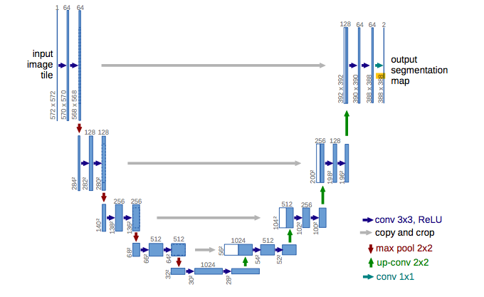
Photo from Ronnenberger et. al, 2015
The Tensorflow website has an excellent example of a U-Net model for binary semantic segmentation which includes data augmentation. This was a good starting point for my toy example. Since I’m dealing with multi class segmentation, we’ll need to make some modification to the code.
The example uses the dice loss function which is common for binary segmentation. For multi class applications we’ll change the loss function to categorical cross entropy. Also we need to change the activation for the final layer to softmax instead of sigmoid.
4. Input data pipeline and creating TFRecords
Optimizing data pipeline in deep learning models is often an overlooked but very important step in getting the best performance. From the Tensorflow website:
“GPUs and TPUs can radically reduce the time required to execute a single training step. Achieving peak performance requires an efficient input pipeline that delivers data for the next step before the current step has finished. The
tf.dataAPI helps to build flexible and efficient input pipelines. “
The Tensorflow example consumes data through the tf.data api and the Dataset.from_tensor_slices() call. tf.data greatly improves the performance and efficiency of reading lots of a data and is the preferred way to get data into your tensorflow model. Although our data set is small and we can fit all the images to memory using Dataset.from_tensor_slices(), I wanted to try using TFRecords. Using TFRecords makes it easier and far more efficient for your Tensorflow model to handle your data, saving it as a sequence of binary strings. It also improves your workflow since you’re left dealing with a handful of TFRecord files vs. hundreds or thousands of image files.
Here are some useful resources on creating an image data pipeline and TFRecords :
- https://cs230-stanford.github.io/tensorflow-input-data.html#building-an-image-data-pipeline
- https://www.tensorflow.org/guide/performance/datasets
- https://www.tensorflow.org/guide/datasets#consuming_tfrecord_data
- https://planspace.org/20170403-images_and_tfrecords/
- http://warmspringwinds.github.io/tensorflow/tf-slim/2016/12/21/tfrecords-guide/
- https://github.com/chiphuyen/stanford-tensorflow-tutorials/blob/master/2017/examples/09_tfrecord_example.py
#Creating a TFRecord, adapted from:
#https://www.tensorflow.org/tutorials/load_data/tf_records
def _bytes_feature(value):
  """Returns a bytes_list from a string / byte."""
  return tf.train.Feature(bytes_list=tf.train.BytesList(value=[value]))

def serialize_example(img,label_img):

    img_str = open(img,'rb').read()
    label_img_str =open(label_img,'rb').read()

    feature = {
        'image':_bytes_feature(img_str),
        'mask':_bytes_feature(label_img_str)
    }

    example_proto = tf.train.Example(features=tf.train.Features\
    (feature=feature))
    return example_proto.SerializeToString()

def tf_serialize_example(img, label_img):
    tf_string = tf.py_func(
        serialize_example,
        (img, label_img),
        tf.string)
    return tf.reshape(tf_string, ())

train_ds = train_ds.map(tf_serialize_example)
val_ds = val_ds.map(tf_serialize_example)
5. Training the Model
I used AWS EC2 to train the model using a P2.xlarge spot instance. I’m sure there are countless tips and tricks to efficiently deal with AWS’ cumbersome interface and connecting to the container using SSH. I found the easiest way for me was to upload my TFrecords to S3 and access the data via my EC2 container. It was very convenient to separate my model script and data for the times when my spot instance expired and I need to fire up another container. For 100 iterations it cost me around $0.50.
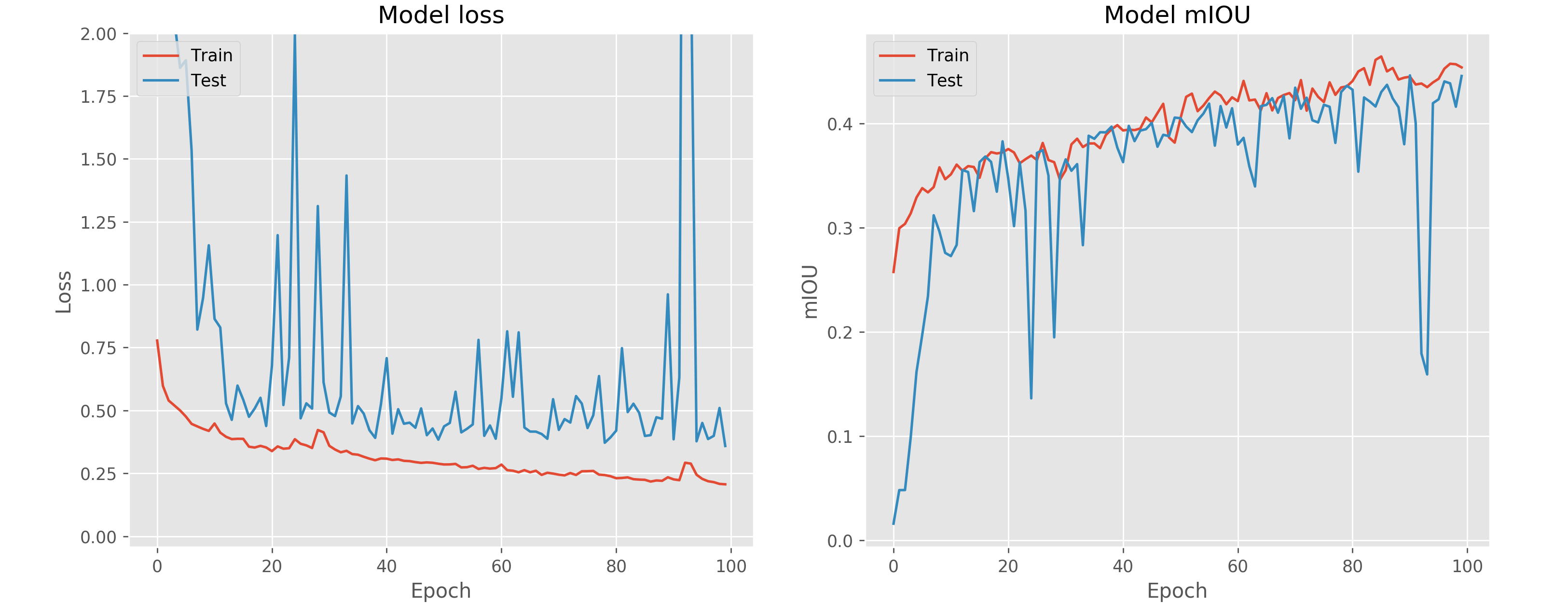
The training metric for semantic segmentation is something important to consider. Typically in journals you will see the “mIOU” as the training metric. This stands for “mean Intersection Over Union” and is a ratio of true positives, false positives, true negatives, and false negatives averaged over all classes in the image. Jeremy Jordan probably has the best explanation of mIOU including some helpful images so I’m going to provide a link to his website.
Using the Keras API makes it little difficult to include custom metrics in the model. Tensorflow has tf.metrics.mean_iou but it’s not easy to include that in your model without some serious hacks. I found this solution to work fine for me.
#adapted from https://www.davidtvs.com/keras-custom-metrics/
class MeanIoU(object):
    def __init__(self, num_classes):
        self.num_classes = num_classes

    def mean_iou(self, y_true, y_pred):
        return tf.py_func(self.np_mean_iou, [y_true, y_pred], tf.float32)

    def np_mean_iou(self, y_true, y_pred):
        target = np.argmax(y_true, axis=-1).ravel()
        predicted = np.argmax(y_pred, axis=-1).ravel()

        x = predicted + self.num_classes * target
        bincount_2d = np.bincount(x.astype(np.int32),\
        minlength=self.num_classes**2)
        assert bincount_2d.size == self.num_classes**2
        conf = bincount_2d.reshape((self.num_classes, self.num_classes))

        true_positive = np.diag(conf)
        false_positive = np.sum(conf, 0) - true_positive
        false_negative = np.sum(conf, 1) - true_positive

        with np.errstate(divide='ignore', invalid='ignore'):
            iou = true_positive / (true_positive + false_positive\
            + false_negative)
        iou[np.isnan(iou)] = 0

        return np.mean(iou).astype(np.float32)

miou_metric = MeanIoU(num_classes)

model.compile(optimizer='adam', loss=losses.categorical_crossentropy,\
metrics=[miou_metric.mean_iou])
The final loss/mIOU charts seem somewhat reasonable for a toy example given that we only have 80 training samples and 20 test samples. Of course we are not expecting to see high performance results with such a small dataset despite some data augmentation.
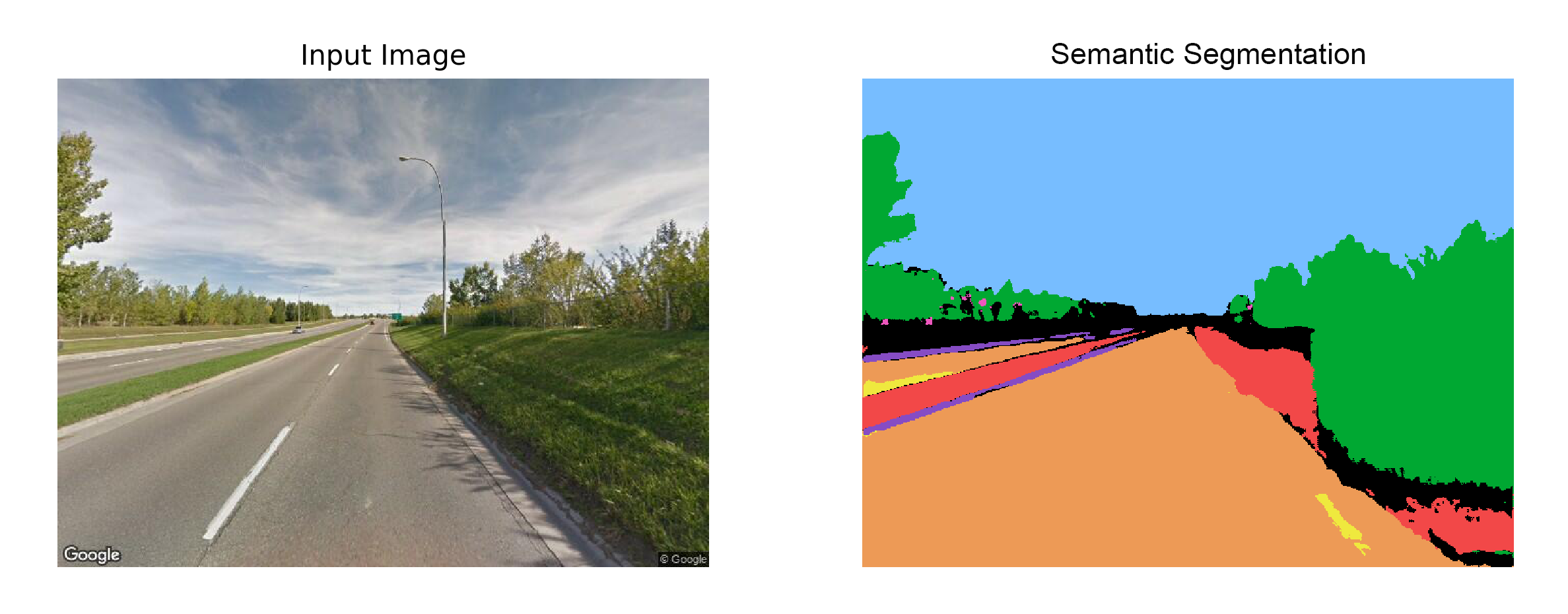
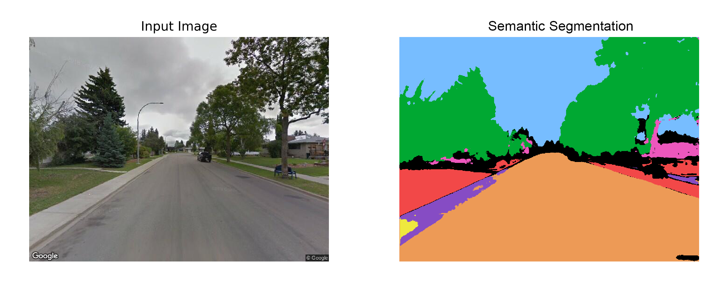
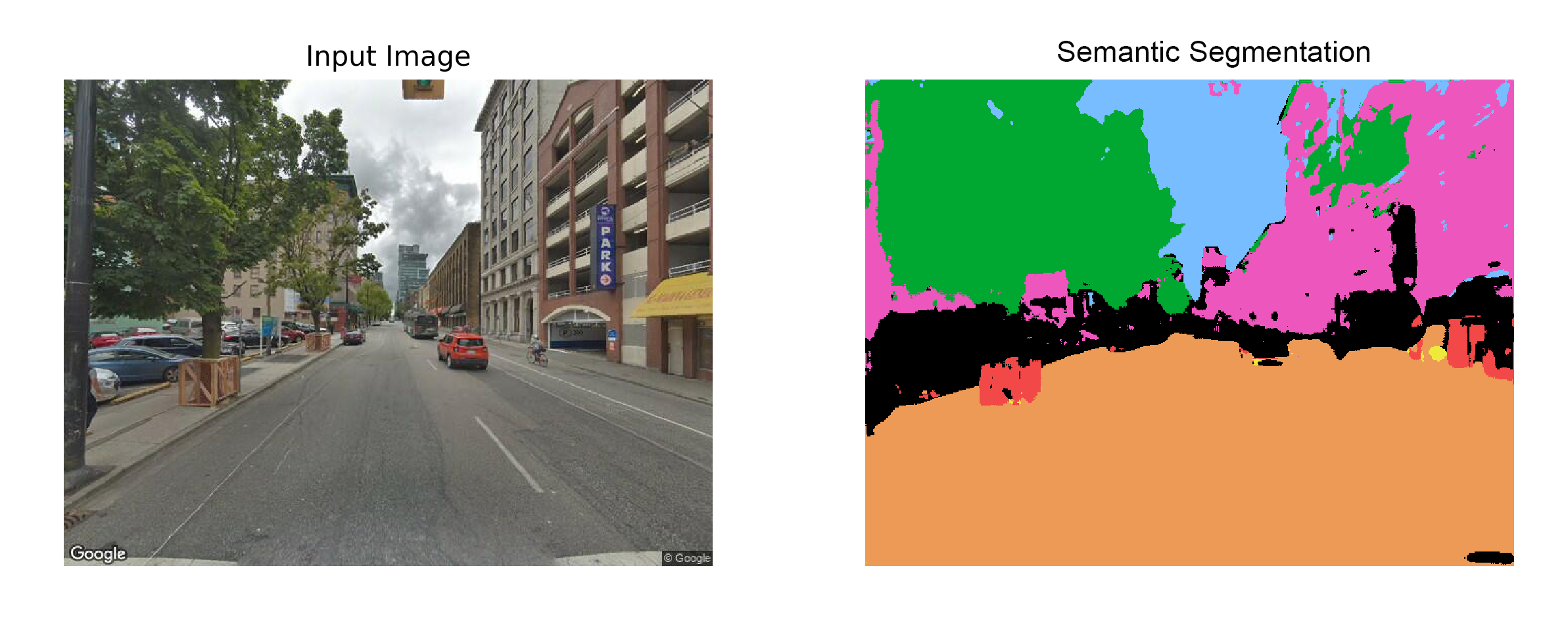
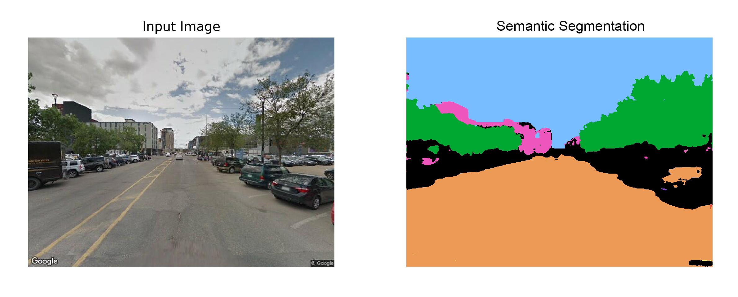
6. Prediction
Finally, lets predict the output masks given some sample images. The output looks acceptable for images with few classes but fails when predicting many classes and complex representations.
References:
- Ronneberger, Olaf; Fischer, Philipp; Brox, Thomas (2015). “U-Net: Convolutional Networks for Biomedical Image Segmentation”. https://arxiv.org/abs/1505.04597